 An official website of the United States government
Developing Public Use Longitudinal Synthetic Microdata with Applications to the Survey of Doctorate Recipients
Disclaimer
Working papers are intended to report exploratory results of research and analysis undertaken by the National Center for Science and Engineering Statistics (NCSES) within the U.S. National Science Foundation (NSF). Any opinions, findings, conclusions, or recommendations expressed in this working paper do not necessarily reflect the views of NSF. This working paper has been released to inform interested parties of ongoing research or activities and to encourage further discussion of the topic.
The Survey of Doctorate Recipients (SDR) public use longitudinal synthetic microdata and corresponding estimates in this working paper are designated as experimental statistical products. These data and estimates are different from and should not be used in place of the longitudinal SDR official statistical products available on the NCSES SDR webpage.
NCSES has reviewed this product for unauthorized disclosure of confidential information and approved its release (NCSES-DRN24-099).
Abstract
In June 2022, the National Center for Science and Engineering Statistics (NCSES) released the restricted use microdata for the longitudinal sample of the Survey of Doctorate Recipients (LSDR) with an InfoBrief on labor force transitions of U.S.-trained doctoral scientists and engineers (Chang et al. 2022). It was the first release of the LSDR panel designed to be maintained through 2025, covering the first three survey cycles of 2015, 2017, and 2019. Research and analytic uses of LSDR data were required in Public Law 117-167 (§10314) and highlighted through recommendations of multiple Committee on National Statistics (CNSTAT) consensus reports (NASEM 2018; NAS, NRC 2014; Fealing, Wyckoff, and Litan 2014). These requirements and recommendations include obtaining longitudinal survey data on the nature, determinants, and consequences of significant transitions in science and engineering career pathways.
A publicly accessible longitudinal microdata file will further address the transparency and reproducibility in statistical information that was recommended in the 2022 CNSTAT consensus study report (NASEM 2022) and will support the tiered access approach noted in the Evidence Act of 2018. This working paper outlines the details of the research conducted to develop public use synthetic microdata for the LSDR data and summarizes the findings from the production phase that led to the construction of the synthetic data file. Synthetic microdata were generated by using a select synthetic data approach. That is, records were partially synthesized, meaning that select variables for select records have been replaced with synthetic values. This working paper includes the rationale behind choosing the selected aspects of synthetic data generation, including the variables synthesized, the extent of synthetic data generation, and the approach for synthetic data generation. The comparison of each option in consideration is described, along with details on the measures used in the comparison. Variance estimation methods are discussed, which allows data users to determine the uncertainty of the estimates.
The public use synthetic microdata for LSDR and corresponding estimates discussed and included in this working paper are designated as experimental statistical products. These experimental statistics may not meet some of NCSES’s quality standards, should not be used to make official statements or inferences about characteristics of the population or economy, and should not be used in place of the LSDR official statistics available on the NCSES SDR Web page. Additional information about the experimental statistical product designation can be found in the Introduction section of this working paper and in the NCSES Statistical Standards.
1. Introduction
The Survey of Doctorate Recipients (SDR) provides biennial individual-level data on policy-relevant characteristics and analytical constructs, including the graduates’ field of study and information relating to employment from a sample of individuals who have earned a research doctorate degree in a science, engineering, or health field from an accredited U.S. academic institution. To increase the analytical benefit of the SDR data, broader access is needed for policymakers, researchers, and other stakeholders to explore the richness of the SDR’s longitudinal structure and inform an increased understanding of career pathways, including higher education, training, work experience, and career development. Toward the goal of broadening data access, the National Center Science and Engineering Statistics (NCSES) within the U.S. National Science Foundation conducted research to assess the feasibility of producing a longitudinal public use synthetic microdata file using the longitudinal sample of the Survey of Doctorate Recipients (LSDR) data from three cycles of the SDR: 2015, 2017, and 2019 (referred to as LSDR 2015–19).
There are a few challenges in producing a longitudinal public use file (L-PUF). One challenge is the balancing of two main goals: (1) maintaining data confidentiality and (2) retaining the integrity of the data. The longitudinal nature of the data adds complexity, as more information is gathered over time for each sampled individual, increasing the risk of disclosure. Furthermore, the existence of cross-sectional public use files (CS-PUFs) provides another source of disclosure risk. It is plausible that a data intruder could link limited data from the L-PUF (fewer variables than on the CS-PUFs) to the CS-PUFs to gather much more information on each individual, again increasing the chances for disclosure. This also raises the possibility that the L-PUF could serve as a bridge to link CS-PUFs across survey years—something that has been difficult to achieve until now—providing survey variables to be used for linking. Another challenge is related to ensuring transparency of the disclosure avoidance approaches and providing the researchers with the means necessary to estimate the precision relating to the statistical estimates.
The main approach used in this research to address disclosure risk is through synthetic data generation with a goal of obtaining analytical outcomes that are consistent with the outcomes that would be produced from the original data. Synthetic data generation involves replacing the original values with synthetic ones generated using statistical or machine learning techniques. These synthetic data sets are constructed to preserve the aggregate statistical properties of the original data set while containing artificial records. The primary argument for generating a synthetic data set as a privacy protection measure is that the records in the synthetic data set do not correspond to any real individuals, allowing the data to be shared and released while minimizing privacy concerns. In the case of partially synthetic data, however, some records may still correspond to actual individuals, although select variables would be replaced with synthetic values. The partially synthetic data approach used in this research and described in detail in this working paper strikes a balance between protecting privacy and preserving the analytical utility of the data.
The public use synthetic microdata for LSDR and corresponding estimates discussed and included in this working paper are designated as experimental statistical products. These experimental statistics may not meet some of NCSES’s quality standards, should not be used to make official statements or inferences about characteristics of the population or economy, and should not be used in place of the LSDR official statistics available on the NCSES SDR Web page. NCSES releases experimental statistical products to benefit users in the absence of other relevant information and to improve future iterations of NCSES data collections. Users should take caution when using the SDR public use longitudinal synthetic estimates presented in this working paper. Additional information about the experimental statistical product designation can be found in the NCSES Statistical Standards.
The work was conducted in two phases:
- A research phase that compared synthetic data approaches to arrive at the recommended approach
- The full development and production phase that produced and evaluated a synthetic longitudinal public use file
Each synthetic data approach implemented in the research phase was designed to retain relationships over time and retain associations between indirect identifiers and the other variables. The research phase focused on a subset of target variables from each cycle. The variables were selected to have different variable types (unordered categorical, ordinal, continuous), and a combination of static and longitudinal variables were selected to be synthesized. To determine suitable synthetic data generation methods, the research explored three approaches, including the model-assisted constrained hotdeck (MACH) method (Krenzke, Li, and Mckenna 2017), a sequential hotdeck approach that builds on the imputation method employed for the longitudinal restricted use file (L-RUF), and the approach of using the open-access R package synthpop (Nowok, Raab, and Dibben 2016). Varying degrees of synthetic data generation were examined as well. For comparison, multiple versions of the synthetic data set were created from the L-RUF for LSDR 2015–19.
The synthetic data approach was chosen based on the best overall results on data utility in the research phase and its expandability to more variables to synthesize in production, while not exceeding a tolerable disclosure risk threshold. The production phase treated many more variables than did the research phase, with the goal being the release of a synthetic L-PUF.
The Methods section (section 2) of this working paper describes the overall research methodology and discusses the following topics:
- Synthetic data approaches used in the research phase
- Variable selection procedures
- Determination process for the records subject to synthetic data generation
- Sampling weight recalibration methods
- Disclosure risk and data utility metrics
- Variance estimation options
The Research Phase section (section 3) of this working paper describes the research conducted comparing the synthetic data approaches, with the goal of determining a recommended approach to use on the production of an L-PUF. It presents the quality control checks and utility measures used to assess the integrity of the synthetic data while accounting for the noise that synthetic data generation introduced. The section includes a comparison of results on the utility of the file, such as a comparison of weighted crosstabs, weighted means, overlapping confidence intervals, and measures of association between the raw and synthetic files. In addition, a summary of some recommendations from the research phase is presented. Finally, the Production Phase section (section 4) of this working paper describes the development and production phase, including the selection of variables to synthesize and the quality control checks that were conducted.
2. Methods
Synthetic data are created through a statistical modeling process to preserve the statistical properties of the original data. The synthetic data approach enables researchers to conduct statistical analyses and obtain results like those from the original data, while keeping the original data confidential. This section covers the methods involved, beginning with the initial disclosure risk assessments, and then delves into the details of the synthetic data generation process, including synthetic data generation methods and the extent of synthetic data generation. Weight recalibration to address discrepancies between the original and synthetic data files is discussed. This section also describes how synthetic data are evaluated in terms of associated disclosure risks and data utility. Finally, the section concludes with a summary of methods for variance estimation.
2.1 Initial Disclosure Risk Assessment
Past disclosure risk assessments (Li, Krenzke, and Li 2022) have shown that a CS-PUF alone has low disclosure risk estimates because it contains limited demographic information. In this research, the authors conducted a matching exercise to the population counts in Survey of Earned Doctorates (SED) table products to identify some SDR subgroups that have high ratios of the sample size to the population size and therefore have high reidentification risk. The risk of correct matching may be low for some of the tables or table cells because the variables—for example, citizenship, marital status, and employment—are time sensitive and can change between a respondent taking the SED and taking the SDR. However, the exercise above informed NCSES that the use of external data sources such as the SED would effectively increase the chance of successful reidentification of SDR respondents by data intruders. To measure the file risk associated with combinations of indirect identifiers, the authors used the model-assisted Skinner and Shlomo (2008) approach, which estimates the probability that a sample unique is unique in the population. At the time, the authors measured the longitudinal risk by linking the 2019 and 2021 SDR CS-PUFs through common variables. The Skinner and Shlomo (2008) approach was utilized to measure the reidentification risk while incorporating the longitudinal nature of the data. This approach measured the increase of longitudinal risk relative to the cross-sectional risk. The model-assisted approach that was adapted to quantify reidentification risk in longitudinal survey data is also provided in Li et al. (2021). Next, to assess the relative risk of respondents, on the basis of k-anonymity, the authors investigated the categories of variables that cause a relatively high risk of disclosure by performing thousands of tabulations that resulted in the identification of unique combinations of variables, categories of variables to collapse, variables to suppress, and data values to target if controlled random treatments (e.g., data swapping, perturbation) are considered. Lastly, the continuous variables were reviewed for outliers that may lead one closer to reidentification.
The L-PUF provides longitudinal information, which can increase the disclosure risk in the CS-PUFs, specifically because of the additional information it would make available beyond what is already included in each publicly available CS-PUF. To quantify the potential increase in risk, the records in the L-RUF 2015–19 were matched to the CS-PUFs for the 2015, 2017, and 2019 cycles, respectively. The matching was based on a set of common variables on each file: 5 static demographic variables, 2 static variables related to the first doctorate, and 29 survey variables on each of the three survey cycles (appendix A).
The L-RUF will not be publicly released; however, this initial assessment identified sample uniques in the L-RUF that can be correctly linked to their corresponding unique records in CS-PUFs. They may require a higher level of synthesis and special handling as they pose elevated disclosure risk across files.
This assessment does not directly measure the risk of a data intruder identifying sampled individuals in the population or identifying correctly and uniquely matching cases to those in the sampling frame. The assessment establishes a baseline for the potential increase in disclosure risk and identifies a broader group of sample uniques that could pose heightened risk if the L-RUF were to be released. The above matching approach measures the chance of getting a correct and unique match between L-RUF and CS-PUFs. Once there is a match, then the reidentification risk of those records is the same or similar to that measured in the case of combined information over years across CS-PUFs in Li, Krenzke, and Li (2022).
To quantify the risk of a data intruder identifying correctly and uniquely matching cases to those in the sampling frame of the SDR, matching was performed between the L-RUF 2015–19 to the sampling frame of the 2015 SDR based on seven common indirect identifier variables. The sampling frame is constructed from the SED data, which have never been publicly available. Although the scenario is unlikely, given that the frame is not publicly available, this examination assessed how likely cases can be reidentified in the population.
2.2 Select Synthetic Data
One may synthesize select records of select variables (Reiter and Kinney 2012) to balance the needs of reducing disclosure risk below a tolerable risk threshold and retaining the integrity of the original data (e.g., maintaining the aggregates, distributions, and associations between variables). In this working paper, this approach is denoted as select synthetic data.
Unlike fully synthetic data (Rubin 1993) and partially synthetic data (Little 1993) in which all records are synthesized for all variables or all records are synthesized for some variables, respectively, records with higher disclosure risks were given a higher chance of being synthesized to effectively reduce the risk while limiting the extent of synthetic data generation, reducing the chance that the integrity of the data is compromised. At the same time, lower-risk records are given a lower chance of being synthesized. This results in keeping a proportion of the original data in the file. Note that all records will have a non-zero chance of being selected for synthesis. Select synthetic data can be considered a form of partially synthetic data.
Mechanically, this approach is implemented by creating risk strata and then randomly selecting records within the strata using a predetermined selection rate, which is referred to as the target treatment rate. To ensure comparability across synthesis methods during the research phase, for each target variable, a set of records was randomly selected to be synthesized using the target treatment rates, and the same set of randomly selected records were synthesized across all three synthesis methods described in the Research Phase section.
During the production phase, all variables in the longitudinal file were considered for synthetic data generation, except for those deemed highly analytically important, such as employment status. In contrast, the research phase focused on a selected subset of variables—encompassing both static and longitudinal variables and all types—for synthesis. A comprehensive list of these variables is provided in appendix A, specifying which variables were synthesized in each phase.
2.3 Synthetic Data Generation Approaches under Consideration
As described in the introduction, this research explored three approaches to creating synthetic data. This section describes and provides an overview of the three approaches: the sequential hotdeck approach, the model-assisted constrained hotdeck (MACH) approach, and the use of the R package synthpop.
2.3.1 Sequential Hotdeck Approach: Extending the SDR Imputation Approach to Synthetic Data Generation
The SDR uses a sequential hotdeck imputation method to address item nonresponse in the cross-sectional data and unit nonresponse in the longitudinal data. Hotdeck imputation is a statistical technique that identifies for each respondent with a missing survey item another respondent (called a donor) with complete data for that item. The complete data are used to impute the missing data. The respondent with the imputed survey data is referred to as a recipient. For each imputed item, donors are selected to match recipients based on specific class variables, so that the respondent who provides the information is similar in that respect to the recipient. Class variables are used to maintain consistency among related variables. For example, Hispanic origin can be used as a class variable for race and ethnicity. As a further step, within a cell, all cases are sorted by sort variables, so that a recipient’s donor is chosen from a respondent nearby according to the sort order. The set of cases with the same values in the full set of class and sort variables is referred to as a cell. The class and sort variables were chosen carefully to minimize nonresponse bias associated with item nonresponse, ensuring a complete data set without missing values for easier data analysis.
Although the goal of imputation differs from the goal of synthetic data generation, the approach leverages the existing method along with carefully selected related variables. For a given static (non-longitudinal) variable, the class and sort variables for a target variable to be synthesized were the first five class and sort variables used for the given target variable in the cross-sectional imputation. The number of class and sort variables were restricted to introduce controlled noise into the selection of the donor, rather than focusing on accuracy. This is to minimize the cases where the same original value might be imputed back to the recipient. For the longitudinal variables, inspired by the longitudinal imputation, the class and sort variables for a variable in a given cycle consisted of the residing location and working status of the three cycles, the corresponding variable in the other cycles (e.g., salary in the 2015 and 2019 cycles to synthesize salary in the 2017 cycle), and the first five class and sort variables used for the given variable in the cross-sectional imputation.
To reflect the uncertainty introduced by synthetic data generation in variance calculations, the process was repeated five times with five bootstrapped samples of donors and relied on the random mechanism of sampling donors with replacement to infuse the variation between implicates (versions of synthesized values).
2.3.2 Model-Assisted Constrained Hotdeck
The MACH approach was influenced by a sequential imputation procedure that was initially designed for handling non-monotone (i.e., Swiss cheese) missing data patterns in complex questionnaires (Judkins et al. 2007) while addressing skip patterns and different variable types. The MACH methodology is described in detail in Krenzke, Li, and McKenna (2017). It has been used successfully to generate synthetic data for the American Community Survey, which is used for the special tabulation for the Census Transportation Planning Products. It has also been demonstrated with the cross sectional 2015 SDR data set for NCSES.
Like the sequential hotdeck approach, the process runs sequentially through each target variable using hotdeck cells. Within each cell, a with-replacement sample from the empirical distribution is conducted to replace each recipient record’s value by another record’s (donor) value. This is carried out for each cell in a single step by replacing original survey values in a random manner.
For each target variable, the hotdeck cells are formed by cross-classifying (1) the target selection flag that indicates the selected records to be replaced; (2) bins created on the target variable to constrain the distance between the original and synthesized values; (3) prediction groups based on the model predicted values (stepwise linear regression for ordinal and continuous variables, and clusters formed from predictions on indicator variables created for unordered categorical variables); (4) auxiliary variables selected to address the need to take account of closely related variables, such as those used in skip patterns; and (5) sampling weight groups based on the magnitude of the weights.
Key features of the MACH include (1) the bounding and control on the amount of noise being added and (2) retaining the association between the target variables and non-target variables by selecting the best predictors from a large pool of variables through a stepwise regression for each target variable. Based on the assignment of the target treatment rates and the variables selected for synthesis, a master index file is used to list the variables to be synthesized as well as the variables to be used as predictors. It also contains all the parameter specifications for hotdeck cell formation and other modeling schemes. The predictions and the subsequent draws from an empirical distribution (hotdeck) occur in a sequential manner (according to the master index file), so that synthetic values are used for the predictor variables in the model for the next variable to be synthesized. The process runs sequentially until all items to be synthesized are processed. In addition, with a goal to incorporate the synthetic data error component, the MACH program was processed five times with a different seed each time to select the target records. For each run, within a cell, a with-replacement sample is drawn, then the sampled values replace the original values for the target variable as implicate 1. In the second run, another with-replacement sample is drawn, and the sampled values are used as implicate 2, and so on. The implicates are then used to account for the additional variabilities introduced from synthetic data generation.
2.3.3 Use of R Package Synthpop
The R package synthpop enables a user to produce synthetic data from original data using various parametric and nonparametric models. The package was produced under the SYLLS (Synthetic Data Estimation for UK Longitudinal Studies) project funded by the UK Economic and Social Research Council. The motivation of the project was to produce synthetic data from UK Longitudinal Studies and share it with researchers after mitigating privacy concerns.
Synthpop is structured to produce partial synthetic data where all the values for a variable are synthesized. The methodology is that of sequential regression modeling. The joint distribution of the observed data is defined in terms of a series of conditional distributions. In a sample of n units consisting of (Xobs,Yobs) where Xobs is a matrix of data that could be released unchanged while Yobs is an n x p matrix of p variables that require synthesis.
An assumption of the synthpop package is that the method of generating the synthetic data (e.g., simple random sample or complex sample design) matches that of the observed data. This allows one to make inferences on synthetic data generated directly from parameters (θ) estimated from the observed data. In other words, the parameters are not drawn from their posterior distributions in the case of parametric models. This is what the package authors call a “simple synthesis” (Nowok, Raab, and Dibben 2016). All the data produced using this package are produced under this assumption. The package provides an option to conduct a “proper synthesis,” where the parameters are sampled from their posterior distributions; however, this was not utilized in this project due to time constraints. More information about synthpop, including a description of the classification and regression trees (CART) and conditional interference trees (CTREE) options mentioned below can be found here: https://cran.r-project.org/web/packages/synthpop/vignettes/synthpop.pdf.
Three types of model classes were used to produce separate synthetic data files:
- CART: Classification and regression trees were used to synthesize all variables in Yobs.
- CTREE and CART: CTREE regression trees were used to synthesize the salary and earning in the 2015, 2017, and 2019 cycles, respectively, and CART was used on the rest of the variables.
- Linear regression and CART: Stepwise linear regression models were used to synthesize the salary and earning in the 2015, 2017, and 2019 cycles, respectively, and CART was used on the rest of the variables.
Three different types of synthetic data were produced using each of the models described above:
- Select synthetic data: Once Yobs was synthesized, only the flagged values under each variable were replaced with their synthesized version.
- Split flagged synthetic data: Here, the original data are subset to just the flagged values and used in model fitting and synthesis. Then the synthesized version is attached back into the original data. The subsetting is performed sequentially for every variable meant for synthesis, as the flags differ from variable to variable. This was also performed for each of the three treatment rate scenarios.
For each type of synthetic data, five implicates were generated by repeating the process five times with different seeds to be used for variance estimation accounting for variabilities due to synthetic data generation.
2.4 Weight Recalibration
The 2015–19 L-RUF underwent weight calibration to align it with known totals, some of which were derived from the sampling frame for the SDR 2015, constructed from the SED data, and some of which were derived from the 2015 cross-sectional restricted use file (CS-RUF) file. Synthetic data generation shifted the weighted distributions for the target synthesized variables. To address this, the weights in the synthetic L-PUF file were calibrated to match the same set of known totals used in weight calibration for the 2015–19 L-RUF. This section details the weight recalibration steps taken after synthetic data generation.
Below is a summary of the process used to create the analysis weights for the 2015–19 synthetic L-PUF file.
- Base weight: A base weight was the final weight of the original 2015–19 L-RUF and was assigned to every case to account for its selection probability under the two-phase sample design and nonresponse in both the 2017 and 2019 cycles. The final weight of the original 2015–19 L-RUF was derived by calibrating its base weight, which is the product of the 2015 SDR final weight and the reciprocal of the probability of inclusion for the longitudinal sample selection. The replicate weights were created using the successive difference replication method (Fay and Train 1995) and underwent a similar calibration process.
- Final weight: Raking adjustments used for the original 2015–19 L-RUF were applied to align the weighted sample distribution in the 2015–19 synthetic L-PUF with known distributions. These known distributions include (1) the population distributions of some key frame variables and (2) the weighted sample distributions of selected control variables in the SDR 2015 file, from which the longitudinal sample was drawn. The variables were selected to support the precision level in the LSDR 2015–19 data tables.
The raking variables are shown in table 1. Following this adjustment, the weight distributions were examined for extreme weights that require trimming. Raking adjustments were then performed on the trimmed weights until the weighted totals conformed to the known totals. The replicate weights were raked similarly, but with control totals including random components to account for the variance in the control totals from the cross sectional 2015 SDR file (see Fuller 1998).
2.5 Disclosure Risk Re-Assessment
To assess the risk remaining in the synthetic data, the matching processes described in Section 2.1 (Initial Disclosure Risk Assessment) were repeated on each synthetic data set. It was anticipated that the matching rate would decline because the synthetic data generation process altered some of the matching variables compared with those in the original data set, thereby reducing the likelihood of correct matches.
2.6 Utility
A list of several utility measures were created to assess how well the synthetic data sets reflect the original 2015–19 L-RUF. The utility measures can be broadly grouped into the following categories:
- Quality control (QC) checks: (1) percentage of records changed and (2) check for atypical value combinations across variables
- Weighted frequency checks: (1) distribution of distances from the original values to the synthesized values, (2) high-utility crosstabs, (3) confidence interval overlap, and (4) confidence interval and point estimation
- Measures of associations checks: (1) pairwise associations, (2) significance of regression coefficients, (3) differences between groups, and (4) U-statistic
- Global utility: (1) visual comparisons of top principal components and (2) change in variable importance in principal component analysis
Many of these utility assessment measures are not applied only to the entire data set but also to specific subgroups.
Each of the above named utility measures are described in further detail below.
2.6.1 QC Checks
The QC utility checks are used to ensure the synthetic data were generated correctly and follow the same logical and skip patterns as the original data. The first QC check utility measure involved calculating the percentage of records changed. For this utility measure, individual crosstabs for each variable were created indicating whether the value was changed in the synthesized data set or not. This utility measure was applied to each treated variable.
The second measure checked for atypical value combinations across variables to confirm that skip patterns present in the original data are also present in the treated data. For a given set of variables, crosstabs were calculated of categorical variables or indicators of whether a variable was missing for both the original and synthetic data sets. Combinations that were in the synthetic data but not the original data were flagged for manual review to confirm it did not violate a skip pattern. Additionally, all possible two-way combinations were exhaustively checked to determine whether variable values were valid, valid skip, or missing.
2.6.2 Weighted Frequency Checks
The first weighted frequency utility measure compared the distance between the original and synthetic values of variables for each individual in the data set. For continuous variables, Euclidean distance was used, and summary statistics of the distances were produced. For categorical variables, Hellinger distance was used. This utility measure checked that the changes for each record and variable were minimal. This measure was applied to each synthesized variable. Part of the checks included comparing the univariate distribution visually through histograms and boxplots.
For combinations of variables considered important, crosstabs were created and the weighted estimate in each cell was compared between the original and synthetic data set. Variable combinations featured in data tables for LSDR 2015–19 (NCSES 2022) were considered important. Since this utility measure can result in many estimates, a plot with the original estimate on the x-axis and the treated estimate on the y-axis was produced to visualize any large deviations. In applying this measure, two sets of variables were used. The first set consisted of derived variables of unemployment spells, employment sector changes, location changes, and working in a field related to the field of doctorate degree. The second set consisted of demographic variables of gender, race and ethnicity, 77-category field of doctorate degree, years since doctorate award, residing location as of 2015, disability status as of 2015, and citizenship status at the time of doctorate award. The derived high-utility crosstabs consisted of three-way crosstabs that included one of the derived variables and two of the demographic variables. The differences between point estimates based on the original and those based on synthetic data relative to the original variance estimates were examined.
For various parameters of importance (e.g., counts, proportions, means) in high-utility crosstabs (LSDR 2015–19 data tables, NCSES 2022), we calculated estimates and confidence intervals using both the original and synthetic data. Ideally, the resulting confidence intervals will mostly overlap so that the same conclusions regarding statistical significance are reached in the synthetic data as in the original data. If the confidence intervals are denoted as (lo, uo) and (ls, us) for the original and synthetic data, respectively, then Karr et al. (2006) calculates the confidence interval overlap as follows:

Furthermore, it was determined whether the estimate using the synthetic data is within the confidence interval obtained using the original data, checking that the estimates from the synthetic data are reasonable given the uncertainty of the original data. Specifically, salary was examined for the 3 years within each race and ethnicity category.
2.6.3 Measure of Association Checks
For variables where fairly high correlations were expected, such as salary over a relatively short time period (e.g., salary in 2015, salary in 2017, and salary in 2019), the correlations between these variables that were maintained in the synthetic data were checked by comparing correlation coefficients. For this set of variables, two correlation matrices were created: one with the original data and one with the synthetic data. To compare the change in the correlations between the original and synthesized data, both absolute change and percent relative change were examined in the correlations. For ordinal variables, the rank correlations were compared between sets of variables using the original data and synthetic data using the same methods as above. All continuous variables (salary, earnings, and weeks worked) for the 3 years were used to measure pairwise associations. A heatmap of correlations and differences in correlations was produced to visually assess which correlations changed and by how much.
When creating synthetic data, the conclusions drawn from regression models using the synthetic data are expected to be similar to those drawn from the original data. For several regression models, the p-values for coefficients obtained from regression models using the synthetic data set were compared with those obtained from the original data. The significance results (at a 0.05 significance level) can be represented in the 2 x 2 contingency table, from which accuracy was calculated—defined as the consistency of significant results.
Statistically significant differences in variables between different demographic subgroups were also checked for consistency. Specifically, outcome variables such as salary and annual raises were examined for racial and ethnic, disabled, and foreign-born subgroups. Ratios of outcome variables were also compared between various subgroups.
2.6.4 Global Utility
Propensity scores were used as a global utility measure for microdata by calculating the U statistic (Woo et al. 2009). To calculate the U statistic, the original and synthetic data are stacked; T = 1 was assigned to the records in the synthetic data, and T = 0 was assigned to records in the original data. A logistic regression model was fitted to T using main effects associated with the synthetic variables. The U statistic was computed as follows:

where n = number of records, = propensity score from logistic regression model for record i, and c = proportion of units from the synthetic data file. U should be close to 0 if the original and synthetic files are indistinguishable. The variance estimate of the U statistic was used from Snoke et al. (2018) to enable statistical testing. The U statistic assesses the multivariate associations between variables in the data and examines whether they are similar in both the original data and synthetic data.
2.7 Variance Estimation
In general, to enable inference from select synthetic data, it is important to release multiple implicates of the synthetic data that accounts for the additional variation resulting from the synthesis process. This section describes how to estimate variances and confidence intervals for estimates of parameters of interests, such as the mean or a regression coefficient, when M implicates of synthetic data are released. However, releasing multiple implicates of synthetic data can increase disclosure risk since not all variables across all records are synthesized and data intruders can pinpoint exactly the variables and their records that had values synthesized.
Therefore, to eliminate the increase to disclosure risk, one could release only one implicate of the synthetic data as it is not evident which records are synthesized. However, releasing only one implicate does not allow for variance estimation that accounts for uncertainty in synthesis which may impact inference. In this section, an approach of using a generalized variance function (GVF) was investigated to allow for variance estimation (Wolter 2007) when releasing only one implicate. A GVF is a regression model that describes the relationship between functions of the variance estimates for estimated population parameters of interest as the dependent variable, and potential independent variables such as the estimate itself and the sample size. Given the need to provide a GVF for every target variable that is synthesized, the limitation of this approach is that data intruders will be aware of which target variables are synthesized. However, the data intruders will not know which of the records of the variables have been synthesized. The GVF approach is discussed further in section 2.7.2, with the recommendation and the adaption of a new approach based on replication weights.
2.7.1 Releasing M Implicates
To obtain proper variance estimates and inference when releasing multiple implicates of synthetic data as briefly described above, it helps to follow the work by Burgette and Reiter (2010). By carrying out the synthetic data generation process multiple times (m = 1,2,…,M), M implicates of synthetic data are created. Let Q be the parameter of interest. For example, the population mean of Y or a regression coefficient of Y on X. For each synthetic data set m, Q is estimated by a point estimate and the variance by . According to Burgette and Reiter (2010), the estimate for Q from the M implicates of synthetic data is and the estimate of the variance V is ū + b/M where the following calculations are needed:


Inference is typically carried out under the t-distribution.
2.7.2 Releasing One Implicate Accompanied with GVFs
Releasing only one implicate has the advantage of preventing data intruders from gaining knowledge of which values are synthesized; however, users are not able to obtain valid inferences that can account for the variability from the synthetic values. In the imputation literature, various correction factors have been proposed to adjust variance estimates, for example, Little and Rubin (1987) and Rubin (1987) calculate a correction factor for the variance of a population mean assuming MCAR (missing completely at random), where is the sample size and the number of imputations, d is small relative to the number of respondents, by: . Note that this simple adjustment factor would not hold under the assumptions for producing select synthetic data. Other approaches under the imputation literature include replication methods. For example, Shao and Sitter (1996) proposed bootstrapping for imputed survey data.
The use of a GVF was investigated for select synthetic data that can inflate variance estimates obtained from a single implicate. Each synthesized variable will need a separate GVF, and as mentioned, data intruders are then informed of which variables are synthesized. Several possible regression models were created to investigate different forms of GVFs that can allow inference in a single implicate of LSDR 2015–19. Conclusions from this investigation showed that the sample size did not affect the inflation in variance significantly for many of the variables investigated, both for the total and within subgroups. Hence, the correction factor to account for the extra variation from the synthesis would be the intercept (a constant). Therefore, releasing one implicate and a series of correction factors for the different variables could be a viable solution to correct for estimating the variances of means and totals. However, as the complexity of the statistical analyses increases, the GVF approach is likely too simplistic a tool, and a conclusion was reached to recommend releasing implicates instead so that analysts can account for the variation arising from the synthesis in their models. It is important to note that releasing implicates can reveal which records have been synthesized, which may increase the risk of disclosure. This potential increase in disclosure risk is briefly addressed in the evaluation presented in the Production Phase section.
2.7.3 Further Perturbing Replicate Weights
To avoid extra computational burden on data users, a different approach was also considered for approximating the variance estimation that is based on stacking the five implicates into one data set and developing replication weights such that they account for the extra variation arising from the synthesis process. Note that this approach provides five times the number of original records based on the five implicates (and therefore the survey weights will be adjusted accordingly) but only includes one vector for each variable. In such a file, the implicate number is not released making it harder to see which variables were synthesized and which records were synthesized. The Production Phase section includes an evaluation for this approach with the theory shown in appendix B.
3. Research Phase
During the research phase, the effects of two factors on synthetic data generation—(1) synthetic data generation methods and (2) the degrees of synthesis—were investigated using multiple experimental settings (three select synthetic approaches crossed with three sets of treatment rates). The results were evaluated and compared in terms of disclosure risk (defined as the likelihood of data intruders gaining additional accurate information about sampled individuals by matching to the respective CS-PUF) and data utility. This section concludes with a summary of the decisions taken on the synthetic data method, treatment rate and approach for proper variance estimation to be implemented in the production phase, which is described in the Production Phase section.
3.1 Initial Risk Assessment
The initial risk assessment revealed that 63% of the L-RUF 2015–19 records were uniquely and correctly matched to their records in all three CS-PUFs even though the L-RUF 2015–19 has a smaller number of survey variables than the cross-sectional files (table 2). It should be noted that the potential for increased disclosure risks due to additional information becoming available was assessed when releasing an L-PUF, given the disclosure risks posed by each publicly available CS-PUF. As mentioned, this assessment does not directly measure the risk of a data intruder identifying sampled individuals in the population or correctly and uniquely identifying matching cases to those in the sampling frame based on SED data. Instead, it establishes a baseline for potential disclosure risk by identifying sample uniques that could pose increased risk if the L-RUF were released. The matching method evaluates the likelihood of correct and unique matches between the L-RUF and CS-PUFs. Once matched, the reidentification risk aligns with that found in previous work on CS-PUFs (Li, Krenzke, and Li 2022). Additional details on the model-assisted approach for estimating reidentification risk in longitudinal data are available in Li et al. (2021). For an example of the risk of disclosure for a publicly available CS-PUF, see Li, Krenzke, and Li (2022).
PUFs = public use files.
Matched records are uniquely and correctly matched for any given matching condition.
National Center for Science and Engineering Statistics, Survey of Doctorate Recipients: Longitudinal Data, 2015–19.
Using seven common indirect identifier variables—age group, place of birth, gender, race and ethnicity, field of study, region of the PhD award institution, and citizenship status at the time of PhD award—approximately 5% of the 2015–19 L-RUF cases were uniquely and correctly matched to their corresponding records in the sampling frame of the cross sectional 2015 SDR sample. This finding suggests that the reidentification risk is relatively low and not a major concern. Notably, the 63% of the L-RUF 2015–19 records that were uniquely and correctly matched to their records in all three CS-PUFs include these 5% of cases uniquely and correctly matched to their respective records in the sample frame.
3.2 Experimental Factors
The effects of two factors on synthetic data generation—(1) synthetic data generation methods and (2) the degrees of synthesis—were evaluated. The three synthetic data generation methods described in the Methods section were used to assess the impact of the data generating method. Additionally, three sets of target amount of data synthesize (referred as treatment rates) were examined to explore how different degrees of synthetic data generation affect disclosure risk and data utility. As outlined in the Methods section, the selected synthetic data were generated using target treatment rates by risk stratum. These rates are detailed in table 3. For consistent comparison, a set of records was randomly selected and synthesized using the target treatment rates for each scenario, and this same set of records was used across all three synthesis methods. In total, nine scenarios (Sequential hotdeck, MACH, synthpop × 82%, 50%, 15%) were analyzed.
CS-PUFs = cross-sectional public use files.
Matched records are uniquely and correctly matched for any given matching condition.
National Center for Science and Engineering Statistics, Survey of Doctorate Recipients: Longitudinal Data, 2015–19.
3.3 Select Variables
As shown in appendix A, a subset of variables was selected to focus on during the research phase and the list of target variables was then expanded for the production phase. The research phase variables were chosen based on needing to represent a variety of situations that are present in the full set of variables in the L-RUF. One situation includes whether the variable is static (does not change over time) or longitudinal. Some variables with strong relationships with other variables were selected. For example, some variables are part of skip patterns. Variables of different types were included, such as unordered categorical, ordinal, and continuous.
3.4 Disclosure Risk Re-Assessment
To assess risk in the synthetic data, the same matching process described in the Methods section was repeated on each of the experimental synthetic data sets. As seen in table 4, the percentage of LSDR 2015–19 cases that were uniquely and correctly matched to all three CS-PUFs decreased from 63% (see table 2) to about 5%, 24%, and 50% for treatment rates of 82%, 50%, and 15%, respectively. The extent of synthetic data generation is the main driving factor in how much risk has been reduced, whereas the synthetic data generation approach did not make meaningful differences.
CS-PUFs = cross-sectional public use files; LSDR = longitudinal sample of the Survey of the Doctorate Recipients; MACH = model-assisted constrained hotdeck.
Matched records are uniquely and correctly matched for any given matching condition.
National Center for Science and Engineering Statistics, Survey of Doctorate Recipients: Longitudinal Data, 2015–19.
The potential increase in risk is not eliminated, but as mentioned in section 3.1, it should be noted that the risk assessment is based on the match rate to the CS-PUFs, serving as a proxy for the potential for increased risk due to additional information released in the longitudinal file. This does not equate to disclosure risk, as a data intruder would still need to link the record to a population file, which would be a worst-case (or arguably unrealistic) scenario where the intruder would have access to the frame file. Therefore, the risk estimates are overstated. Nonetheless, these measures are useful to help understand the potential reduction in risk.
For the matching to the sampling frame, as in the initial disclosure risk assessment, seven common indirect identifier variables were used for matching: age group, place of birth, gender, race and ethnicity, field of study, region of the PhD award institution, and citizenship status at the time of PhD award. The matching rate was decreased from 5% to about 1%, 3%, and 4% for treatment rates of 82%, 50%, and 15%, respectively.
The risk assessment indicates that the synthetic data generation process has considerably reduced the risks associated with the original data.
3.5 Checks and Utility
Using the utility measures as specified in the Methods section, each of the synthesis methods and treatment rates received a ranking according to each measure. This required each utility measure to be summarized with a single number that summarizes how well the utility measure performed across each of the five implicates for a given treatment. How the rankings were derived for each of the utility measures are described below.
For each of the synthetic continuous variables, each method was ranked by the weighted difference in means between the original and synthetic values, using the weight in the original data (L-RUF). Then, the ranks for each approach were averaged and re-ranked according to the average ranks of the individual variables. The ranks for categorical variables were constructed similarly but using the Hellinger distance instead of the weighted mean.
For the high-utility crosstabs (LSDR 2015–19 data tables), each approach was ranked according to the mean relative absolute difference between the weighted cell total for the original and synthetic data set.
Rankings were created for the confidence interval overlap and indicator for whether the synthetic estimate was located within the original confidence interval at the 95% confidence level according to their respective means. That is, mean of the IO (calculated using the formula given in section 2.6.2) was computed for each variable as well as the percentage of synthesized estimates that were within the original confidence intervals.
The ranking for pairwise associations was determined by taking the mean relative absolute difference of each of the pairwise correlations. For the significance of regression coefficients, the mean consistency of significance of the regression coefficients was considered across implicates for the synthetic data compared with the original data. If a coefficient is statistically significant at the 0.05 significance level (p < 0.05) in both data sets or not significant (p ≥ 0.05) in each data set, it is considered consistent. Lastly, the mean p-value was used across implicates for each treatment for the U statistic (the larger the better).
The 24 options were compared (three treatment rates of 82%, 50%, and 15% crossed with eight synthetic data generation approaches of sequential hotdeck, MACH, and six combinations of synthpop), and table 5 displays the rankings, in which 1 indicates the best option and 24 the worst. The ratios of each utility measure value to the corresponding value for the sequential hotdeck approach at a treatment rate of 15%, which resulted in the best utility overall, are shown in table 6. Both tables illustrate that the treatment rates have a greater impact on utility, compared with the synthetic data generation approaches (e.g., sequential hotdeck vs. MACH). The ranking suggests that the sequential hotdeck approach outperformed the others, followed very closely by MACH, with the combinations of synthpop approaches coming last. The results highlight the potential benefits of leveraging a process tailored for LSDR.
Y = yes.
CART = classification and regression trees; CTREE = conditional interference trees; LinReg = linear regression; MACH = model-assisted constrained hotdeck.
Ranking value 1 indicates the best option and 24 indicates the worst.
Y = yes.
CART = classification and regression trees; CTREE = conditional interference trees; LinReg = linear regression; MACH = model-assisted constrained hotdeck.
Figure 1 presents a risk-utility plot. The x-axis represents the risk, measured as the percentage of LSDR 2015–19 cases that are uniquely and correctly matched to all three CS-PUFs (table 4), whereas the y-axis represents utility, measured as the average ratio of utility measures to the corresponding measure for the sequential hotdeck approach with an overall synthesis rate of 15% (table 6), across different utility measures. This approach served as the benchmark, as it produced the highest overall utility. To ensure consistency in the interpretation of utility metrics, all measures were transformed so that lower values indicate better utility. For example, metrics indicating closeness (e.g., confidence interval overlap) were converted into measures of distance (e.g., confidence interval non-overlap), and proportions of consistent statistical conclusions were recast as proportions of inconsistent conclusions. The results from the synthpop approach are displayed, specifically from the select synthesis “Synthpop LinReg/CART” option, as it performed the best among all the synthpop combinations.
CART = classification and regression trees; CS-PUFs = cross-sectional public use files; LinReg = linear regression; LSDR = longitudinal sample of the Survey of the Doctorate Recipients; MACH = model-assisted constrained hotdeck.
All utility measures were converted to represent distance, with smaller values indicating better utility.
In figure 1, it is evident that treatment rates have a considerable impact on both risk and utility, more so than the choice of synthetic data generation approach. Although the performance and utility of all three approaches are comparable within a specific treatment rate scenario, the sequential hotdeck and MACH approaches consistently preserved the integrity of the original data slightly better than the synthpop approach.
Given that disclosure risk is defined as the extra information gained by releasing an LSDR data set together with their CS-PUF counterparts, the 50% treatment scenario was found to introduce sufficient uncertainty to mitigate this risk. In terms of data utility, the 50% treatment scenario outperforms the scenario with higher treatment rates. As shown in figure 1, the sequential hotdeck or MACH approach under the 50% treatment scenario falls closest to the bottom-left quadrant of the risk-utility plot—representing lower risk and higher utility—and thus provides the best balance between reducing risk and maintaining data integrity. It should also be factored in that the two approaches consistently demonstrated higher data utility across various evaluation metrics.
Figure 2 compares the weighted percentage of individuals with no changes in employer sector across all three cycles in the original data against the same estimates in two synthetic data sets: one using the MACH approach and the other using the sequential hotdeck approach; both approaches in the figure used scenario 2, with an overall treatment rate of 50%. The figures display estimates by sex, race and ethnicity, field of degree, and years since doctorate award, as well as the residing location, disability status, and citizenship status as of 2015. Estimates from both synthetic data sets are very close to the original ones with estimates from the MACH approach being slightly closer (average absolute difference of 0.19% vs. 0.21%). This is an example of how well the data integrity was preserved in this particular set of synthesized longitudinal variables, aided by weight recalibration.
MACH = model-assisted constrained hotdeck.
3.6 Summary of Research Phase and Selection of Synthetic Data Approach
Uses of synthetic data have been consistently increasing as the demand for access to microdata and privacy concerns grows. For example, synthetic data are seen as a solution for sharing vast amounts of health data toward developing machine learning models and speeding up research on health data while protecting privacy (e.g., Synthea, as detailed in Walonoski et al. 2018). Challenges to generating synthetic data are balancing the reduction of disclosure risk with retaining the integrity of the original data (e.g., maintaining the aggregates, distributions, and associations between variables). To address these challenges, one may synthesize a select set of variables and select records with high disclosure risks, referred to as the “select” synthetic data approach. Three main select synthetic data approaches were applied to the L-RUF for LSDR 2015–19. In this section, a summary is provided of the synthetic data approaches, treatment rates, variance estimation approaches, and decisions made for production based on the findings from the research phase.
Finding 1 (synthetic data generation approach). The MACH approach was selected to produce an L-PUF for LSDR 2015–19.
Each of the three approaches used a hotdeck cell approach to replace original data. The first approach, referred to as the sequential hotdeck approach, is an expansion of the imputation approach tailored to the SDR longitudinal data, taking advantage of existing imputation cells that account for various associations. The second approach, MACH, constrains the distance from the original value and uses predicted mean matching from a main effects model in the formulation of the hotdeck cells. The third approach includes variations of the R package synthpop, including the CART option which forms hotdeck cells under a model with varying degrees of interaction terms, finding the most important effects on the target variable.
Conceptually, the sequential hotdeck approach can be applied to other data sets; however, it would need to be tailored to each specific data set, especially if the imputation process is not already in place. The MACH approach, on the other hand, can be seamlessly applied to any synthetic data generating application as it is parameter-driven. Although the synthpop approaches use open-source code and can be readily used for other applications to other data sets, it does not give users much control over the modeling process (e.g., users cannot force predictors into the model) and needs tailoring for some options (e.g., parametric regression options require predictors to be selected beforehand).
A thorough and systematic evaluation was conducted to find the best among three approaches. Considering disclosure risk reduction, retention of data utility, and ability to apply to different situations, the best approach was determined to be the MACH approach. The method is developed for synthetic data generation, which conducts a built-in model selection process and synthetic data generation and resulted in the best or the second-best utility in the experiment and similar risk results as other methods. The imputation method performed well for continuous variables mainly because the correlations among salary (or earning) in three different cycles are well-maintained. This was done by systematically respecting longitudinal patterns. For example, to synthesize the salary variable in the 2017 cycle, the salary variable in the 2015 and 2019 cycles were the key variables used in forming imputation cells. This type of tailoring was incorporated into the MACH approach as post-synthesis edits, building on what we have learned from the research phase. Table 7 compares the features of the three synthetic data generation methods, highlighting that the MACH and synthpop method provides capabilities for synthetic data generation such variable selection and modeling.
MACH = model-assisted constrained hotdeck.
Finding 2 (treatment rate). The medium treatment rate (overall rate of 50%) was selected to balance risk reduction with retaining data integrity.
Three target treatment rates (proportion of records synthesized) were employed during the research: high (overall rate of 82%), medium (overall rate of 50%), and low (overall rate of 15%). The research results were as expected. They showed that the higher the target treatment rate, the greater the risk reduction (with respect to mitigating the additional information gained by releasing a L-PUF together with cross-sectional counterparts) and the lower the data utility. The authors determined that a 5% reduction in the distance between the original data and synthetic data (increase in utility) across various aspects is worthwhile.
Finding 3 (variable estimation method). To appropriately reflect the variability introduced by synthetic data generation, multiple implicates will be released, rather than the GVF approach that uses only one implicate and correction factors. This was due to the limitation that the GVF approach is too simplistic to allow for more complex modelling. Although the risk reduction due to the synthesizing is not fully realized due to a data intruder knowing which values were synthesized, it allows users to account for the variance component introduced by synthetic data generation in all their analyses.
In general, an estimate of the total variance should account for the synthetic data variance component. Each of the approaches for generating synthetic data has a way of accounting for this term through multiple imputation. The imputation and synthpop approaches repeated the process five times and relied on the random mechanism to infuse the variation between implicates. For the MACH approach, a bootstrap sample of donors was selected within each hotdeck cell. The process was repeated five times.
For the research phase’s recommended approach (MACH), the percentage of the total variance attributable to the synthetic data variance term is 5% to 20% across the three levels of treatment rates. Because the variance term is not negligible, there needs to be a way for users to account for this term in the synthetic public use file (L-PUF). The multiple implicates approach provides a data intruder two pieces of information that some agencies have traditionally suppressed from public knowledge. For one, if the variable has implicates, a data intruder knows which variables were synthesized. Furthermore, if variability exists among the implicates for a given record, then a data intruder knows that those records were synthesized. Therefore, if multiple implicates exist on the file, a data intruder will know the variables and the records that were synthesized. There is some risk in this; however, the intruder will not know the original values. Also, releasing the implicates allows the users to account for the synthetic data error variance component for all types of analyses. The user manual will provide guidelines for using implicates for accurate variance estimation in various statistical programming languages.
4. Production Phase
This section describes the process of creating and evaluating the L-PUF for LSDR 2015–19. The research phase concluded that the MACH approach would be used to create the L-RUF with an overall treatment rate of 50%. More details on the MACH approach are provided in this section.
The variables to be synthesized (i.e., target variables) were expanded as indicated in appendix A. In addition, several derived variables were synthesized indirectly by being re-derived from synthesized variables. Besides synthesized variables, the L-PUF also includes some variables in their original values since they have important analytical value or low disclosure risk, e.g., whether an individual lives in the United States, job code for principal job in major field of study in minor groups. These variables are considered analytically important because they are consistently utilized in NCSES publications for their relevance and value in analysis.
4.1 Implementation
The synthetic data generation process is managed through a Master Index File (MIF). The MIF specifies the variables to be synthesized, the partial treatment rates (i.e., the percentage of records to be synthesized) for each risk stratum, and the variables to be included in the pool of candidate predictor variables. It also classifies each variable into one of three types: real numeric, ordered categorical, or unordered categorical. For unordered categorical variables, indicator variables were created. Key features of MACH’s process include:
- Partial treatment rates: These rates were determined based on research phase findings to ensure that approximately 50% of the records were synthesized overall. The partial replacement rates were set at 0.61, 0.41, 0.20, and 0.02 for the four risk strata, from highest risk to lowest risk, as defined in table 2. With the overall rate of 50% and a minimum rate of 2%, the stratum-level replacement rate was determined so that the rates for the second and third strata are approximately one-third and one-sixth of the rate for the riskiest stratum. Although this is somewhat arbitrary, it reflects the structure used to determine the replacement rates at the stratum level.
- Target selection flag: Each variable’s target selection flag was set individually. The flag was set to one if the associated data value was selected for synthesis through a random process. This process involved randomly selecting records based on the partial treatment rate within each risk stratum. Records were sorted by the target variable and key analysis domains, including 5-year award groups for first U.S. science, engineering, or health PhD; gender; race and ethnicity; work status; and residence in the United States, to ensure synthesis occurred across the values of these variables.
- Variable preparation: Predictor variables were recoded as needed for model selection. This step also compiled the pool of predictor variables and created indicator variables for unordered categorical variables.
- Model selection and prediction: After variable preparation, model selection was performed to identify predictors for each target variable and estimate model parameters for generating predicted values. These predicted values were essential for creating hotdeck cells in the synthesis step. The model selection and prediction were done once for each variable using the L-RUF, as the joint distribution among the variables is already given in the original data.
- Hotdeck cells: Hotdeck cells were formed for each target variable by cross-classifying (1) target selection flags indicating records to be replaced, (2) bins created on the target variable to constrain the distance between original and synthesized values, (3) prediction groups based on model predictions (e.g., stepwise linear regression for ordinal and continuous variables, clusters for unordered categorical variables), (4) auxiliary variables accounting for closely related variables, and (5) sampling weight groups. Small cells (cells size less than three) were identified and combined automatically. The five components of the hotdeck cells were sorted in a serpentine manner, and if a cell had fewer respondents than a pre-assigned threshold, it was collapsed with the preceding cell. The rank order of the second to fourth components could be tailored for each target variable via the MIF.
- Synthesis: Target variables were synthesized by drawing from the empirical distribution within each hotdeck cell, without replacement. The approach is model-assisted, utilizing parameters from the model selection process to generate predicted values for forming hotdeck cells.
- Drawing and updating: Within each final hotdeck cell, a with-replacement draw was conducted. Target records were identified by their partial replacement flag, and values were replaced through random draws with replacement from the empirical distribution within the hotdeck cell. Records not targeted for replacement did not contribute values.
- Sequential processing: The predictions and subsequent draws occurred sequentially, with synthetic values used for predictor variables in models for the next variable to be synthesized. Target variables were ordered on the MIF so that those most likely to be predictors were synthesized earlier. The process ran sequentially through all items flagged for synthesis.
- Post-processing checks: After synthesis, pre- and post-synthesis checks were performed to assess the impact, including generating frequencies, means, and correlations before and after synthesis.
The entire process was repeated five times independently with different seeds, resulting in five versions of synthesized values, or implicates.
4.2 Evaluation
This section evaluates the resulting select synthetic data generated using the selected factors: the MACH approach and a synthesis rate of 50% in terms of disclosure risk (defined as the likelihood of data intruders gaining additional accurate information about sampled individuals by matching to the respective cross-sectional PUF) and data utility.
4.2.1 Disclosure Risk Re-Assessment
To assess risk in the synthetic data, the same matching process described in the Methods section was repeated on the synthetic data set. As seen in table 8, the percentage of LSDR 2015–19 cases that were uniquely and correctly matched to all three, two, and one CS-PUFs decreased from 63%, 24%, and 6% to 0%, 1%, and 5%, respectively. If a case was matched to a CS-PUF using one implicate, it was considered matched to be conservative. This implies that the 2015–19 synthetic L-PUF poses minimal risk of providing further information than what is already publicly available in the three CS-PUFs. For example, publicly releasing the 2015–19 synthetic L-PUF would not allow data users to link CS-PUFs to append more longitudinal information.
CS-PUFs = cross-sectional public use files; PUFs = public use files; LSDR = longitudinal sample of the Survey of the Doctorate Recipients.
Using the seven common indirect identifier variables listed in sections 2.1, 3.1, and 3.4, the percentage of LSDR 2015–19 cases that were uniquely and correctly matched to the sampling frame was relatively low at about 5% in the 2015–19 L-RUF, and it decreased even further to less than 1% in the 2015–19 synthetic PUF across implicates. While releasing the implicates may increase disclosure risk by indicating which records are likely to be original, the low matching rate suggests that this is unlikely to pose a significant concern.
The risk assessment indicates that the synthetic data generation process has considerably reduced the risks associated with the original data.
4.2.2 Checks and Utility
The utility metrics outlined in the Methods section were used to evaluate the utility of the resulting synthetic data.
- Percentage of records changed: As the number of variables subject to synthetic data generation increased to 93, all the LSDR 2015–19 cases had at least one variable with its value changed. Table 9 presents the number of cases by the number of variables (out of 93) with any changes in at least one implicate. The effect of this distribution, with the spread of synthesis across many variables and all records having at least one changed value, is shown in the substantial risk reduction seen in table 8.
- A typical value combinations across variables: Through exhaustively checking all possible two-way combinations of whether variable values were valid, valid skip, or missing, it was confirmed that the skip patterns present in the original data are maintained in the synthetic data.
- Distance between original and synthetic values: For the 15 continuous variables—SDRAYR, SDRYR; AGE_15; WKSWK_15, _17, _19; TENYR_15, _17, _19; SALARY_15, 17, 19; and EARN_15, 17, 19—Euclidean distances between the original data and the synthetic data were calculated and then standardized using the standard error of the original data. The standardized Euclidean distances ranged from 1% to 25%. The largest distance is observed in the tenure year reported in the 2019 cycle. On average, the difference between the synthetic tenure year and the original tenure year is about 0.07 among all tenured individuals, indicating that the synthetic data closely aligns with the original data.
- Distance between distributions by original data and by synthetic data: For categorical variables, Hellinger distance, measuring the difference between two univariate probability distribution was calculated. The Hellinger distances ranged from 0 to 0.02. The largest distance is seen in the marital status in 2019, with the percentage of married individuals shifting from 80.71% to 80.47%. This change, however, does not reveal any substantial differences in the distribution of categorical variables.
- Weighted estimate checks: As described in the Methods section, high utility crosstabs were used, which consisted of three-way crosstabs involving one of the key outcome variables and two demographic variables. The key outcome variables were unemployment spells, sector changes, and location changes, and working in a field related to the field of doctorate degree. The first three are longitudinal. The demographic variables were gender, race and ethnicity, 26-category field of doctorate degree, years since doctorate award, residing location as of 2015, disability status as of 2015, and citizenship status at the time of doctorate award. The estimates were for totals, proportions, the median salary of three cycles, and the median changes in salary (from 2015 to 2019).
- Measures of associations checks: The correlation between SDRYR and AGE and the correlations between salary in different cycles and earnings in different cycles were well-preserved, with more slight decreases than slight increases (as expected) (table 10). Cases with valid skips or top coding were excluded from the calculation.
Out of 64,692 estimates in 10,782 cells, the standardized distance (the difference between the estimate using the original data and the estimate using the synthetic data relative to the original standard error) ranged from 0% to 52%.
Confidence intervals for the same 64,692 estimates were created and the overlap ranged from 25% to 97%. The largest distance and the smallest overlap came from a small cell in a table involving sector changes by race and ethnicity and disability status. Among the synthetic point estimates, 92% were included in their corresponding confidence intervals using the original data.
Regression models were developed for salary in three cycles with age, race and ethnicity indicators, whether living with children, and employer sectors as covariates. Out of 45 regression coefficients, 2 had inconsistencies in the statistical conclusion at a 0.05 significance level. For pay increases from 2015 to 2019, out of 15, 1 had a difference in the statistical conclusion. More changes were present for smaller subgroups such as non-Hispanic Black, disabled, and foreign-born subgroups.
4.3 Variance Estimation
As mentioned, all implicates of the synthetic data will be released to allow for proper variance estimation. Under the replication weights approach, the five implicates are stacked, resulting in a file that has five records for each person. The survey weights aligned with each record are divided by five to retain the total sum of weights. As outlined in appendix B, the variance estimation method is based on replication weights, which were further perturbed to account for variance introduced by synthetic data generation. This method was evaluated by comparing its variance estimates with those derived from the combining rule in Reiter and Kinney (2012). Specifically, two sets of variance estimates were compared for the 64,692 estimates in the high-utility crosstabs used in the data utility evaluation. The average ratio of the two variance estimates was 1, with values ranging from 0.91 to 1.12, and the distribution was closely centered around this average.
5. Conclusion
The results from the disclosure risk analysis by Li, Krenzke, and Li (2022) show that the disclosure risk for the 2021 cross-sectional PUF was considered low, especially after confidentiality treatments were implemented (e.g., variable suppression, recoding). This result was consistent with a similar analysis done for the 2019 CS PUF. In addition, recognizing the SDR panel has been in the survey for multiple years, some protective measures were implemented to reduce the risk of combining CS-PUFs over time so data intruders could not gather additional information about individuals in the sample.
There has been much interest in the longitudinal information that SDR collects. The information has been accessible through restricted access. To provide the data more broadly, a PUF version of the longitudinal data has been considered. However, having more information about individuals, such as employment status, marital status, and other identifying variables that can change over time, increases disclosure risk. One approach is to limit the number of variables in a longitudinal PUF; however, it has been shown that a small number of longitudinal identifying variables have a good chance to match uniquely and correctly to the CS-PUFs. If a data intruder is able to successfully do that match, it would open up a large pool of variables gathered on those matched individuals. Li, Krenzke, and Li (2022) showed that introducing a longitudinal structure increased the disclosure risk by a factor of five.
From these prior disclosure risk assessments, it is clear that a synthetic L-PUF is needed to be able to reduce the risk of matching to the CS-PUFs and subsequently putting together a longitudinal data record for the successful matches. The goal of the synthetic data approach is to reduce the disclosure risk while creating a file that retains data utility—that is, the file would be analytically useful. To that end, a select synthetic approach was used where a subset of variables were synthesized for a subset of data records, where the chance of synthesis was applied differentially depending on the disclosure risk of the records. Three main approaches were evaluated, including a sequential hotdeck, model-assisted constrained hotdeck (MACH), and variations of the R package synthpop, including the CART option that forms hotdeck cells under a model with varying degrees of interaction terms. The results showed a slight edge to moving forward to the production phase with the MACH approach based on disclosure risk reduction, retention of data utility, and ability to apply to different situations. In addition, the treatment rate (synthesis rate) was determined through a risk-utility map. Lastly, a new variance estimation approach for synthetic data on complex samples was developed (see appendix B). The variance estimation approach modifies the replicate weights to account for multiple implicates stacked within the data set. As a result, the resulting file includes all implicates generated from the synthetic data process for each variable along with the corresponding replicate weights. This structure makes the synthetic data transparent to the user while informing the user of the precision of the estimates, which includes the variance component due to the synthetic data process.
The MACH was implemented successfully to produce a 2015–19 synthetic L-PUF. The synthetic L-PUF was checked for disclosure risk, and the results show that there is minimal chance that publicly releasing the 2015–19 synthetic L-PUF would allow data users to link CS-PUFs to append more longitudinal information. Furthermore, several data utility checks were reviewed. The published tables from the LSDR were compared with the tables generated from the synthetic L-PUF without any concern noted. This is likely due to the weight calibration step that was applied after the data were synthesized. Results from other tables matched well. Regression model results were also reviewed and were mainly consistent (e.g., 3 of 60 regression coefficients would lead to different analytical conclusions). More inconsistencies were found when looking at subgroups such as foreign born, disabilities, and non-Hispanic Black.
In conclusion, it should be cautioned that not every combination of variables or analytical approach was checked for consistency. However, among the data checked, the approach that was applied resulted in a mix of synthetic and original data in the file. This approach gave a better chance of creating an analytically useful file. The synthetic L-PUF can be useful for researchers to gain insights into the SDR population.
Although this method provides a solid foundation, it is not exhaustive and can—and should—be expanded as the field of synthetic data generation continues to evolve. A potential direction for future synthetic data generation efforts is outlined in appendix C, which highlights recent advancements in the field that could be applicable to LSDR.
References
Andridge RR, Little RJA. 2010. A Review of Hot Deck Imputation for Survey Non-Response. International Statistical Review 78(1):40-64.
Burgette LF, Reiter JP. 2010. Multiple Imputation for Missing Data via Sequential Regression Trees. American Journal of Epidemiology 172(9):1070–76.
Chang W-Y, Wang Y, Milan L, Foley D; National Center for Science and Engineering Statistics (NCSES). 2022. Labor Force Transitions of U.S.-Trained Doctoral Scientists and Engineers: Findings from a New Longitudinal Panel. InfoBrief NSF 22-327. Alexandria, VA: U.S. National Science Foundation. Available at https://ncses.nsf.gov/pubs/nsf22327/.
Fay R, Train G. 1995. Aspects of Survey and Model-Based Postcensal Estimation of Income and Poverty Characteristics for States and Counties. Proceedings of the Section on Government Statistics. Alexandria, VA: American Statistical Association, pp. 154−59.
Fealing KH, Wyckoff AW, Litan RE, editors. 2014. Capturing Change in Science, Technology, and Innovation: Improving Indicators to Inform Policy. National Academies Press. Available at https://nap.nationalacademies.org/resource/18606/dbasse_160935.pdf.
Fuller WA. 1998. Replication Variance Estimation for Two-Phase Samples. Statistica Sinica 8(4):1153–64.
Judkins D, Piesse A, Krenzke T, Fan Z, Haung WC. 2007. Preservation of Skip Patterns and Covariance Structure through Semi-Parametric Whole-Questionnaire Imputation. Joint Statistical Meetings Proceedings of the Section on Survey Research Methods of the American Statistical Association.
Karami H, Atienza D, Ionescu A. 2024. SynEHRgy: Synthesizing Mixed-Type Structured Electronic Health Records Using Decoder-Only Transformers. arXiv preprint arXiv:2411.13428.
Karr AF, Kohnen CN, Oganian A, Reiter JP, Sanil AP. 2006. A Framework for Evaluating the Utility of Data Altered to Protect Confidentiality. The American Statistician 60:224–32.
Krenzke T, Li J, Mckenna L. 2017. Producing Multiple Tables for Small Areas with Confidentiality Protection. Journal of the International Association of Official Statistics 33(2):469–85. Available at https://doi.org/10.3233/SJI-160259.
Li L, Krenzke T, Li J. 2022. Risk Assessment on 2021 Survey of Doctoral Recipients Public Use File. Technical report prepared for the National Center for Science and Engineering Statistics (NCSES). For more information, contact NCSES, https://ncses.nsf.gov/surveys/doctorate-recipients/.
Li J, Li L, Krenzke T, Chang W-Y. 2021. An Approach to Estimate the Re-Identification Risk in Longitudinal Survey Microdata. Proceedings of the Survey Research Methods Section. Alexandria, VA: American Statistical Association, pp. 1837–42.
Little RJA, Rubin DB. 1987. Statistical Analysis with Missing Data. New York: Wiley.
Little RJA. 1993. Statistical Analysis of Masked Data. Journal of Official Statistics 9:407–26.
National Academies of Sciences, National Research Council (NAS, NRC). 2014. The Past, Present, and Future of Federal Surveys: Observations from the Committee on National Statistics. Available at http://www-stat.wharton.upenn.edu/~lbrown/Papers/2014i%20JSM%20Proceedings%20-%20CNSTAT%20review%20of%20federal%20surveys%20-%20final.pdf.
National Academies of Sciences, Engineering, and Medicine (NASEM). 2018. Measuring the 21st Century Science and Engineering Workforce Population: Evolving Needs. Washington, DC: The National Academies Press. Available at https://doi.org/10.17226/24968.
National Academies of Sciences, Engineering, and Medicine (NASEM). 2022. Transparency in Statistical Information for the National Center for Science and Engineering Statistics and All Federal Statistical Agencies. Washington, DC: The National Academies Press. Available at https://doi.org/10.17226/26360.
National Center for Science and Engineering Statistics (NCSES). 2022. Survey of Doctorate Recipients, Longitudinal Data: 2015–19. NSF 22-326. Alexandria, VA: U.S. National Science Foundation. Available at https://ncses.nsf.gov/pubs/nsf22326/.
Nowok B, Raab GM, Dibben C. 2016. synthpop: Bespoke Creation of Synthetic Data in R. Journal of Statistical Software 74(11):1–26. Available at https://doi.org/10.18637/jss.v074.i11.
Pang C, Jiang X, Kalluri K, Spotnitz M, Chen R, Perotte A, Natarajan K. 2021. CEHR-BERT: Incorporating Temporal Information from Structured EHR Data to Improve Prediction Tasks. Proceedings of Machine Learning for Health 158:239–60.
Reiter JP, Kinney SK. 2012. Inferentially valid partially synthetic data: Generating from posterior predictive distributions not necessary. Journal of Official Statistics. 28:583–590.
Rubin DB. 1987. Multiple Imputation for Nonresponse in Surveys. New York: John Wiley and Sons.
Rubin DB. 1993. Discussion: Statistical disclosure limitation. Journal of Official Statistics 9:462–68.
Skinner C, Shlomo N. 2008. Assessing Identification Risk in Survey Microdata Using Log-Linear Models. Journal of the American Statistical Association 103(483):989–1001.
Shao J, Sitter RR. 1996. Bootstrap for Imputed Survey Data. Journal of the American Statistical Association 91(435):1278–88.
Snoke J, Raab G, Nowok B, Dibben C, Slavkovic A. 2018. General and specific utility measures for synthetic data. Journal of the Royal Statistical Society. Series A: Statistics in Society. 181(3):663–88.
Walonoski J, Kramer M, Nichols J, Quina A, Moesel C, Hall D, Duffett C, Dube K, Gallagher T, McLachlan S. 2018. Synthea: An Approach, Method, and Software Mechanism for Generating Synthetic Patients and the Synthetic Electronic Health Care Record. Journal of the American Medical Informatics Association 25(3):230–38.
Wolter KM. 2007. Chapter 7: Generalized Variance Functions. Introduction to Variance Estimation, 2nd ed. New York, NY, Springer.
Woo M, Reiter J, Oganian A, Karr A. 2009. Global measures of data utility for microdata masked for disclosure limitation. Journal of Privacy and Confidentiality. 1(1):111–24.
Notes
1 See the technical notes for the National Center for Science and Engineering Statistics (NCSES). 2022. Survey of Doctorate Recipients, Longitudinal Data: 2015–19. NSF 22-326. Alexandria, VA: U.S. National Science Foundation. Available at https://ncses.nsf.gov/pubs/nsf22326#technical-notes.
2 See the data tables for National Center for Science and Engineering Statistics (NCSES). 2021. Survey of Doctorate Recipients, 2019. NSF 21-320. Alexandria, VA: U.S. National Science Foundation. Available at https://ncses.nsf.gov/surveys/doctorate-recipients/2021#data.
3 The approach uses the predictive mean to form prediction groups to use in constructing hotdeck cells, along similar lines to a method described by Andridge and Little (2010).
4 See the Data Tables for National Center for Science and Engineering Statistics (NCSES). 2022. Survey of Doctorate Recipients, Longitudinal Data: 2015–19. NSF 22-326. Alexandria, VA: U.S. National Science Foundation. Available at https://ncses.nsf.gov/pubs/nsf22326#data-tables.
5 This type of comparison can be expanded in the final documentation if needed.
6 Select interaction effects can be specified.
Suggested Citation
National Center for Science and Engineering Statistics. 2025. Developing Public Use Longitudinal Synthetic Microdata with Applications to the Survey of Doctorate Recipients. Working Paper NCSES 25-221. Alexandria, VA: U.S. National Science Foundation. Available at https://ncses.nsf.gov/pubs/ncses25221.
Contact Us
National Center for Science and Engineering Statistics
Directorate for Social, Behavioral and Economic Sciences
U.S. National Science Foundation
Alexandria, VA 22314
Tel: (703) 292-8780
FIRS: (800) 877-8339
TDD: (800) 281-8749
E-mail: ncsesweb@nsf.gov
Appendix A: Variable List
DRF = Doctorate Records File; TOD = taxonomy of disciplines.
Appendix B: Replicate Weight Perturbation for Synthetic Data
Let and represent the design and unit nonresponse mechanism and the synthetic data generation mechanism, respectively.
Let and , where

K is the number of implicates, su is the set of indices of records with observed values, and st is the set of indices of records with synthesized values.
Assuming

This can be estimated by

where

n is the sample size, and is the r-th base replicate weight of unit i for the longitudinal sample of the Survey of Doctorate Recipients (LSDR) 2015–19 synthetic public use file, which is the r-th final replicate weight of unit i for the LSDR 2015–19 restricted use file.
where .
where for .
is the replication variance estimator ignoring synthetic data generation.

As the expectation of with respect to the synthetic data generation mechanism is zero,

Various solutions can be found to

For the LSDR, K = 5. As some LSDR’s key estimates are not smooth and analysts may want to study a small population, zeroing out or doubling should be avoided. A solution can be found by setting and , .

In the LSDR, d ≈ 2.5 and , where .
Out of 104 replicate weights, the first R = 50 replicates weights were further perturbed (then and ), where
Appendix C: Potential Future Uses of Artificial Intelligence Methods for Synthetic Data Generation
For future work, it may be worth considering the use of artificial intelligence methods, particularly large language models (LLMs) for synthetic data generation. LLMs for synthetic data generation have been successfully employed in the area of electronic health records (EHR) with examples including CEHR-GPT (Pang et al. 2021) and SynEHRgy (Karami, Atienza, and Ionescu 2024). While the longitudinal sample of Survey of Doctorate Recipients (LSDR) does not involve health records, much of this work is directly translatable, as the data are of similar structure (e.g., longitudinal structure). These models provide a number of advantages over more traditional methods. In particular, instead of relying on rigid assumptions, they are extremely flexible with respect to modeling underlying marginal and joint distributions of variables. Secondly, they are able to perform partial synthesis and capture both cross-sectional and longitudinal information in a natural way.
While LLMs are most commonly applied to natural language, they can be applied to structured longitudinal data. Both CEHR-GPT and SynEHRgy create semi-structured sequences of varying length from structured longitudinal data. These sequences can be seen as “sentences,” comprehensible by the underlying architecture of LLMs such as GPT. The approach of CEHR-GPT is to use cross-sectional data (either generated by CEHR-GPT itself or another method) as a “prompt” with GPT producing responses in the form of synthetic longitudinal information. However, these sentences are not examples of natural language, which means the extensive pretraining over large corpuses found among popular LLM models would not be able to be leveraged, but it would be possible to train a version of LLM over LSDR data, as did the authors of CEHR-GPT and SynEHRgy with other data sets.
These methods are open source, but they are not in the form that can be used for LSDR without modification. In particular, the available code to convert raw data to and from sequences presume particular EHR data formats. That component would need to be replaced with customized code to do the appropriate conversions. However, the code to model and produce synthetic sequences are capable of modeling sequences produced by different types of data, so should not require much, if any, adjustment.
A potentially greater challenge in implementing this approach successfully is that it does not directly optimize risk or utility metrics, and in the case that the resulting data set fails with respect to one or more of these metrics, the fixes are not obvious—certainly not a matter of tweaking a parameter. If there are concerns after running risk and utility assessments, the use of acceptance-rejection methods that target the metrics could be investigated. Fortunately, this may not be necessary as prior research indicates that LMM approaches scores well in terms of both disclosure risk and data utility without special adjustments. The authors of SynEHRgy claim it outperformed other sophisticated methods for prediction, and there were not any identified privacy risks. CEHR-GPT performed similarly.
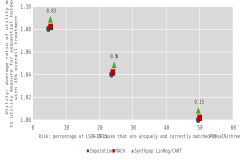
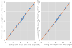
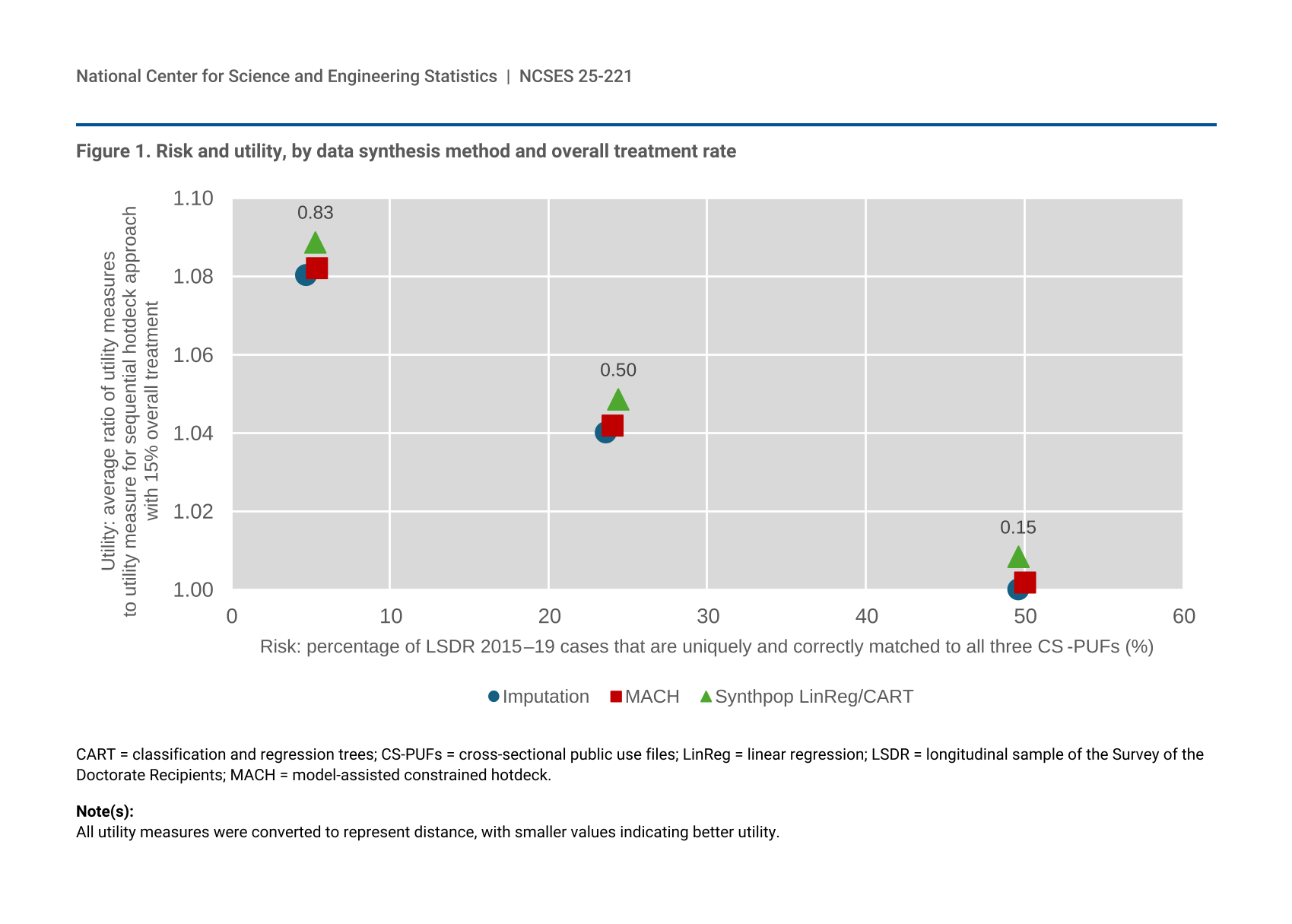